

26 January 2023
26 January 2023
Simulation methodology

To simulate the high resolution data of MTG/FCI polar satellite data are used. A schematic representation of the processing steps is shown in Figure 1. Depending on the case, VIIRS, MODIS and/or AVHRR data are used. GOES/ABI data are used to demonstrate how data comparable to FCI performs polar satellite data. Parallax shift is not simulated, but the difference in viewing geometry is shown with comparison images from SEVIRI or GOES/ABI. In addition to MTG/FCI, MSG/SEVIRI instrument data are also simulated so that the methodology can be compared against actual SEVIRI data.
Transforming polar data to geostationary SEVIRI data
For simulating MSG/SEVIRI, the polar satellite data are collected to the SEVIRI 3km sub-satellite point grid using bucket resampling (middle image in Figure 1). In this method all polar satellite pixels that are within one SEVIRI pixel are averaged. This method leaves some holes (missing data) where no polar data are coinciding with the SEVIRI grid.
Transforming polar data to geostationary FCI data
As a first step, the polar satellite data are resampled to a grid that would correspond to the FCI instrument at 250m sub-satellite resolution using nearest neighbour resampling. This data are then aggregated to the actual resolution of the FCI channel in question, by taking an average suitable grouping of the pixels. Both nominal and high resolution modes can be used for the channels that have both distribution modes.
The bucket resampling approach isn't used due to the high resolution of the FCI instrument. The selected approach will provide a good estimate without leaving any missing data in the images.
Target area imagery
The target area images are resampled from the intermediate data in geostationary projection using bilinear interpolation with gradient search algorithm for fast resampling. The target image resolutions are selected so they would best demonstrate the instrument resolution.
In addition to simulated SEVIRI and FCI images, the original polar data are resampled directly to the target area to further give references.
Limitations of the method
Simulating future satellite instrument imagery is very complex if all influencing factors are considered. In practice, there are two ways to approach this issue (e.g. Schmit et al 2005). One way is to utilise radiative transfer model calculations, the other is to use existing satellite data. This simulation uses existing satellite data. The methodology used in the simulator only takes into account the change in the resolution of the images. Therefore, the simulator has limitations that should be kept in mind when viewing images. The issues related to the properties of the instruments, including measurement angle and the transfer of radiation from surface or clouds to instrument, affects to final 'real' image. In this simulation these factors are not applied to the simulations due to its complexity. Below is a brief introduction on these matters and references for further reading.
Instrument properties
Each satellite instrument measures the radiation differently. For different applications, meteorological satellite instruments measures atmospheric and surface properties through different channels, carefully selected parts of the visible and infrared electromagnetic spectrum. The spectral response function (SRF) of an instrument describes its relative sensitivity to energy of different wavelengths. When an instrument has its own spectral response functions, there may be differences in the colours of RGB images, when comparing the simulated image (Figure 2b) with the observed one (Figure 2a). Below is an example from the case study Dense fog over southern Finland.


There are also additional factors that make visible differences in simulated images. Zhang et al (2006) has described the factors in instrument that has blurring influence on image quality in following way:
For an ideal instrument, the detector output is proportional to the pixel radiance within footprint i.e., the geometrical field of view (GFOV). However, real instruments do not exactly reproduce the spatial radiance field of the pixel; a nontrivial portion of the energy comes from the surrounding area. This energy from outside the GFOV introduces the blurring influence, which degrades the image quality.
Diffraction is one of the unavoidable factors that generate a blurring influence. Diffraction in a satellite sensor occurs because the diameter of the optical system has a limited size. It reduces the detector response from the radiances within the GFOV and increases its response from the radiances outside the GFOV. Other factors, such as the time response of the detector, electronics (analog-to-digital conversion), scan pattern,atmospheric effects, as well as image resampling can cause additional blurring influence
Because of the high orbital altitude, an instrument on a geostationary satellite (GEO) has a larger blurring.
Further information
Schmit et al (2005): Introducing the next-generation Advanced Baseline Imager on GOES-R, https://doi.org/10.1175/BAMS-86-8-1079
Zhang et al (2006): Impact of Point Spread Function on Infrared Radiances From Geostationary Satellites, https://doi.org/10.1109/TGRS.2006.872096
Instrument pixel geometries

In polar satellite instrument scanning geometry also affects on the spatial coverage and shape of the pixel. Difference between instruments is most visible at the edge of the swath as can been seen from the Figure 3.
Further information
Visible Infrared Imaging Radiometer Suite (VIIRS) Imagery Environmental Data Record (EDR) user's guide: https://doi.org/10.7289/V5/TR-NESDIS-150, page 13, Figure 7
Miller, Sh., K. Grant and J. J. Puschell (2013a): VIIRS Improvements Over MODIS. 2013 EUMETSAT Meteorological Satellite Conference and 19 th AMS Satellite Meteorology, Oceanography and Climatology Conference. Vienna, Austria, 16-20 September 2013.
COMET Module Introduction to VIIRS Imaging and Applications
Geometrical effects
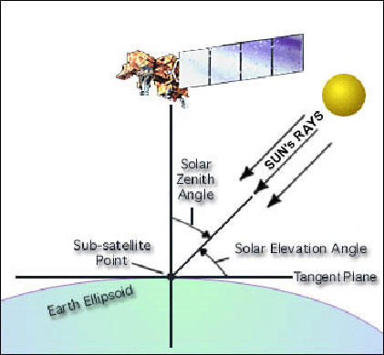
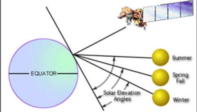
Geostationary satellite viewing angle does not change with time, because satellite is situated in a fixed location. In the case of polar satellites, viewing angles changes as a satellite moves along its orbital path. The solar and satellite viewing directions significantly influence satellite measurement when sun elevation is low (Figure 4b). This affects the calculated RGB composite, so the same composite could look very different for LEO compared to GEO. From late autumn to early spring, when the solar elevation angle is very low at high latitudes, GEO satellite measurements are more often saturated than LEO satellites due to unfavorable sun-satellite geometry.
Examples in Figure 5a and b, from the case study Freezing precipitation at Helsinki-Vantaa airport


Parallax effects
When the satellite viewing angle is away from the sub-satellite point (nadir), an object’s position is shifted (Figure 6a & b). Displacement grows more quickly with increasing distance from the nadir. At large viewing angles, high clouds move further than low clouds and the distortion of the shape of the original feature is also greater. At very slated view, the satellite actually measures the side of clouds rather than the top.


On Figure 6a the small red circle at top of the imaginary 'overgrown' storm represents, for example, an overshooting top. The two red dotted lines indicate the apparent location of this feature, as observed from two different places in space — one representing a nadir view (e.g. from a satellite in polar orbit, with the storm at its swath centre), and the other a view from a geostationary satellite. While the nadir view places the feature properly, at its real location, the slant view from the geostationary position shifts the apparent location of the feature significantly northward (up in this drawing) with respect to the real position of the feature. This difference in apparent location of the feature (indicated by the thick red double arrow) is called the 'parallax shift'.
On Figure 6b the two red dotted lines indicate the edges of the image swath, the longer dotted blue line its centre (nadir view, centre of the satellite swath). The thick red double arrow indicates the parallax shift for a storm further away from the swath centre.
Parallax shift and shape degradation affects both GEO and LEO satellites. As polar satellites orbit is at a much lower altitude than geostationary satellites, resolution is much better at high latitudes and also cloud displacement is negligible near the nadir. Despite this, it is worth keeping in mind that for lower orbits the viewing angle and parallax displacement grows more quickly with increasing distance from nadir (Figure 7). At the edge of the swath, especially high Cb clouds are displaced relative to the surface but also a semi-transparent cloud appears thicker because the measurement reaching the satellite took a longer path through it.

Further information
The Problem With Parallax: Part 1-3
Limb cooling
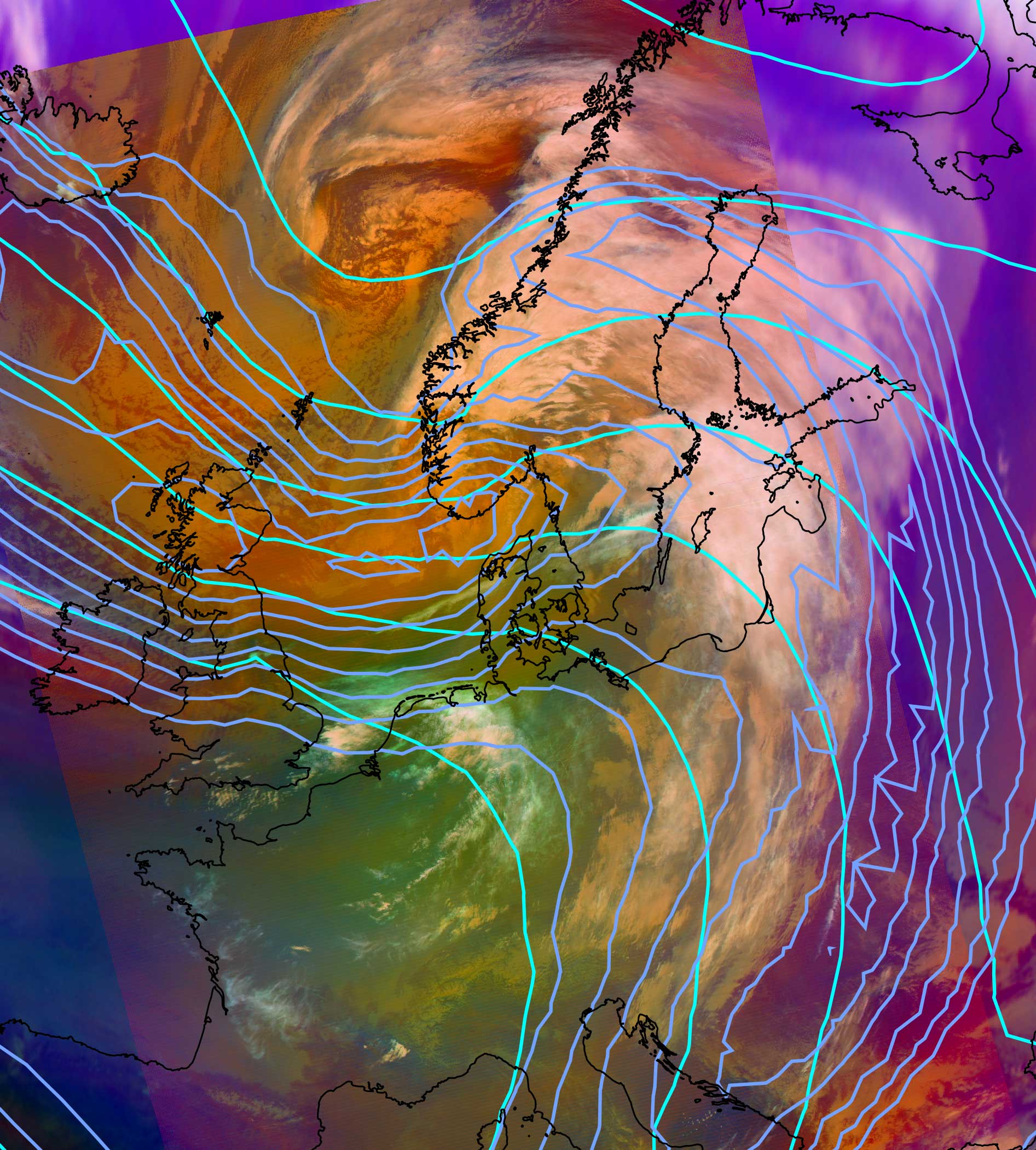
The limb-cooling is a result of an increase in measurement (optical) path length of the absorbing atmosphere, as viewing zenith angle increases (see this NASA technical report). Major absorbing variables are water vapour, ozone and carbon dioxide. Satellite instrument IR measurements are colder at locations that are far from sub-satellite point (nadir). This affects RGB composite interpretation by causing anomalous reductions in brightness temperature, thus especially changing the colour interpretation of the water vapour RGB composites. Example from the case study Development of storm Valtteri (Figure 8).
Further information
Instructions for using the simulator
Limb cooling effect (EUMeTrain)