16 February 2023
22 December 2020
System Vicarious Calibration (SVC) of Ocean Colour (OC) sensors is required, along with instrumental calibration, to meet stringent accuracy requirements of the water-leaving radiance products and all downstream bio-optical products.
Water-leaving radiance forms just a small portion of the radiance measured by the sensor at the top of atmosphere (TOA). The OC-SVC method inherently considers system from the sensor and the Level-2 processing chain and TOA radiometry up to the marine signal, as one entity. In essence, it consists of computing the expected TOA radiometry, that results from both the physics embedded in the processor (radiative transfer modelling) and high-quality sea-truth measurements concurrent, with space acquisitions from the visible (VIS) to the near-infrared (NIR) part of the solar spectrum. Individual SVC gains are then classically defined as the ratio between the expected and actual TOA radiances at each match-up and each relevant wavelength, and are finally averaged over the mission life-time. In practice, the individual gains are computed, such that they make the system exactly match the in-situ measurement. The gains are, therefore, intrinsic to a given system, and operational agencies in charge of OC dataset must be able to update them after any evolution of the Level-1 and Level-2 processing chain.
Objectives
The overall purpose of the study was to deliver a tool that computes, in an easy and traceable manner, the OC-SVC gains required by EUMETSAT in its daily operation of OC missions.
The detailed objectives of the study were to:
- Review the OC requirements for SVC gains generation.
- Propose a versatile method able to handle any OC sensor and processing chain.
- Develop and test the software tool (SW-TOOL).
- Support the installation of the SW-TOOL on EUMETSAT Offline Environment and organise on-site training courses.
- Achieve a real demonstration (DEMO-TOOL) with the generation of SVC gains for Sentinel-3 OLCI-A and OLCI-B data (EUMETSAT reprocessing of 2020/2021, collection 003).
- Assess the impact of the SVC gains.
- Document exhaustively the software and the demonstration (DOC-TOOL).
Overview
Requirements for SVC
The protocols and methods used in the Ocean Colour community for SVC have been summarised and have contributed to the design of the SW-TOOL:
- Criteria to filter the match-up database (MDB): flags, thresholds, statistical screening.
- SVC procedure, in particular as defined for standard atmospheric correction (e.g., visible/NIR sequential computation).
- Post-processing: protocols for gains averaging and further analysis of individual gains.
Generic SVC method
To handle any Level-2 processor, the remote-sensing reflectance provided by the Level-2 processor at m bands is formally expressed as a function of the gains through:
For a given match-up, the SVC is defined as an optimal problem: find a spectral gain g=(g1,g2,⋯,gn ) for calibration of n bands at TOA, which minimises the discrepancy between the retrieved Rrs and targeted Rtrs given by sea-truth measurement, defined by following χ2 cost function:

The numerical computation of the individual gains relies thus on an iterative algorithm, running the Level-2 processor as a black-box and minimising this discrepancy. The method currently implemented in the SW-TOOL can be interpreted as the first iteration of the Gauss-Newton algorithm and retrieves exactly the standard gain computation when applied to standard atmospheric correction. For instance, for OLCI processing chain, the marine reflectance in the visible is given after application of gains on a pre-corrected TOA reflectance ρgc:
In this case, the solution of the SW-TOOL converges toward the known explicit formulation of Franz et al. (2007), involving the target marine reflectance ρtw (in the geometry of the sensor), path reflectance ρpath and transmittance t, these latter being considered as the reference after a NIR calibration is done beforehand:
The method is described in the ATBD section of the DOC-TOOL.
Software development
The SW-TOOL is fully developed in Python 3 and distributed directly in source code on the EUMETSAT Gitlab server. It is operated through a Graphical User Interface (GUI, see Figure 1) giving access to two main functionalities:
- The computation of individual SVC gains over a match-up database (MDB) between satellite data and high quality in-situ marine reflectance.
- The post-processing and analysis of these individual gains, up to the provision of mission average gains which shall be applied in operation.
A third functionality is an optional pre-processing of the database, to restrict its coverage before running the SVC and speed up the processing to only useful match-ups.

An important feature of the software design is traceability: each run of the SW-TOOL (pre-processing, gains computation, post-processing) generates an output configuration file summarising exhaustively the data and options selected by the user.
For being versatile, the process handles separately the Level-1 MDB and the corresponding archive of Level-1b Processing Distribution Units (PDUs) stored on the user disk space, both being univocally linked through the PDU filenames registered in the MDB. The Level-2 processor is assumed to process the Level-1 PDUs in their native format (specific to the sensor), while the SW-TOOL deals only in a generic way the MDB. The Level-2 processor is invoked as a black-box by a so-called wrapper, using a pre-defined list of required arguments handled by the SW-TOOL and possibly other specific options/arguments for the given processor (Figure 2).
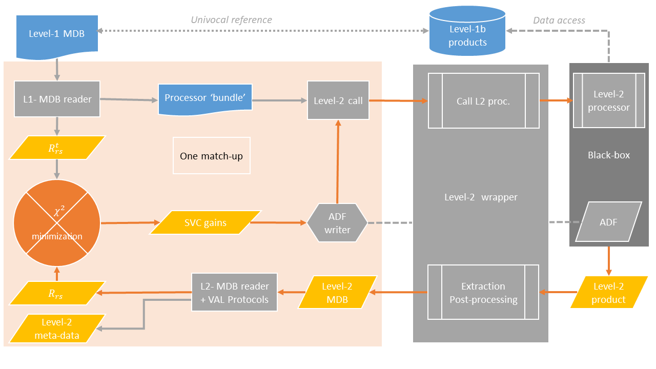
Due to the non-standard implementation of the SVC computation as an iterative method, it is important to check the relevance of the individual gains. For this, the SW-TOOL applies the individual gains at TOA, launches one more time the Level-2 processor and plots the satellite marine reflectance against the targeted values. For standard AC, the individual SVC shall make the satellite data perfectly match the in-situ measurements (Figure 3, right).

Demonstration for OLCI-A & OLCI-B
After having computed SVC gains in the NIR over the South Pacific Gyre (SPG), the demonstration has required a complete review of the MOBY database for gains in the visible:
- Hyperspectral measurements were integrated over OLCI-A/B spectral response functions.
- Only post-deployments calibrations were selected.
- The selection of radiometric data at sea-surface with respect to depth propagation followed a prioritisation logic agreed with MOBY team: Lw21 > Lw22 > Lw1 > Lw2.
- Good and Questionable data were kept to maximise number of match-ups, seasonality and overlap between OLCI-A and OLCI-B.

Table 1. Statistics of OLCI-A (left) and OLCI-B (right) averaged gains at MOBY (400 to 681nm) and SPG (709 to 1020nm), after MSIQR filtering.
| Band | OLCI-A matchup number | OLCI-A Average gain | OLCI-A standard deviation | OLCI-A RSEM (%) | OLCI-B matchup number | OLCI-B Average gain | OLCI-B standard deviation | OLCI-B RSEM (%) |
|---|---|---|---|---|---|---|---|---|
| 400 | 42 | 0.975458 | 0.005544 | 0.0517 | 19 | 0.994584 | 0.004464 | 0.0339 |
| 412.5 | 42 | 0.974061 | 0.005897 | 0.0551 | 19 | 0.9901 | 0.003902 | 0.0297 |
| 442.5 | 42 | 0.974919 | 0.005435 | 0.0507 | 19 | 0.992215 | 0.004418 | 0.0336 |
| 490 | 42 | 0.968897 | 0.005645 | 0.053 | 19 | 0.986199 | 0.004067 | 0.0311 |
| 510 | 42 | 0.971844 | 0.004139 | 0.0388 | 19 | 0.988985 | 0.003604 | 0.0275 |
| 560 | 42 | 0.975705 | 0.003086 | 0.0288 | 19 | 0.99114 | 0.003021 | 0.023 |
| 620 | 42 | 0.980013 | 0.002107 | 0.0196 | 19 | 0.997689 | 0.002244 | 0.017 |
| 665 | 42 | 0.978339 | 0.001412 | 0.0131 | 19 | 0.996837 | 0.001841 | 0.0139 |
| 673.75 | 42 | 0.978597 | 0.002128 | 0.0198 | 19 | 0.997165 | 0.001695 | 0.0128 |
| 681.25 | 42 | 0.979083 | 0.001504 | 0.014 | 19 | 0.998016 | 0.001902 | 0.0144 |
| 708.75 | 27 | 0.980135 | 0.004555 | 14 | 0.997824 | 0.003089 | ||
| 753.75 | 27 | 0.985516 | 0.003723 | 14 | 1.001631 | 0.002391 | ||
| 778.75 | 27 | 0.987718 | 0.00352 | 14 | 1.002586 | 0.002176 | ||
| 865 | 0.986 | 1 | ||||||
| 885 | 27 | 0.986569 | 0.00176 | 14 | 1.000891 | 0.001693 | ||
| 1020 | 27 | 0.913161 | 0.008537 | 14 | 0.940641 | 0.007011 |
Gains were found to have an excellent temporal stability at all bands, with variation in the blue bands likely linked to the seasonal variation of the actual in situ measurement at this bands where the signal is the strongest, and to be robust to geometry and detectors. An interesting indicator implemented in the SW-TOOL to check the suitability of gains with respect to stability requirement in ocean colour (0.5% on marine reflectance over a decade) is the Relative Standard Error of the Mean (RSEM) proposed by Zibordi et al. (2015). It is computed at a given band λi by:

where ḡ is the mean gain, σ the standard-deviation of the individual gains and Ny the number of individual gains (i.e. good match-ups), scaled over a decade (i.e. Ny=10 N/Y where N and Y are the actual number of match-ups and measurement years, respectively). Values of RSEM for OLCI-A and OLCI-B, scalded over a decade (Table 1 and Figure 5, bottom) reach closely the requirements, being as low as 0.05% in the blue and nearly 0.025% at 560nm; they decrease in the red toward 0.01%, however without reaching the target of 0.005% that seems unachievable over clear waters with such methodology.

Impact assessment
To assess the impact of gains, EUMETSAT launched the IPF on match-ups and generated Level-3 products at global scale over various type waters (oligotrophic, mesotrophic and eutrophic waters). The main effect of SVC gains that can be observed relatively independently of other Level-2 algorithmic evolutions is the excellent consistency between OLCI-A and OLCI-B ocean colour radiometry over clear waters. While previous processing baseline PB 2.23 presented more than 10% relative differences in marine reflectance (Figure 6, top), the new processor with SW-TOOL gains has managed to align the sensors’ radiometry within 2.5% or even less at all bands in the blue and green (Figure 6, bottom, for 412 nm). This exercise demonstrates the benefit of the SW-TOOL to get a consistent SVC process for data harmonisation: harmonised database of high-quality in-situ data, with harmonised protocols and process.