L1C co-registration algorithm for 3MI

The multi-viewing, multi-channel and multi-polarisation Imager (3MI) on board the Metop-SG satellites will observe polarised multi-spectral radiances of a single target, within a very short time range, from the visible to the short-wave infrared region with daily global coverage.

Objectives

The objective of the L1C co-registration algorithm is to produce a geo-projected and re-gridded radiance product from the 3MI sensed data and, in addition, to co-locate ancillary information, in particular from the METimage 20-channel imager, providing sub-pixel information of the radiance field and clouds.

Overview

Users of 3MI level-1 radiance data for the retrieval of geophysical properties will often need to relate multiple 3MI measurements to a given geo-location for all spectral channels, the three Stokes vector components and for the full range of available observation geometries. Since this co-registration of the temporal sequence of 3MI radiances is not straight-forward, there is a clear need to make such data available in a well-defined way along with complete characterisation of the involved re-gridding errors. At the same time, the multi-dimensionality of such data calls for a user-friendly geo-located product including ancillary data like terrain height or ancillary information from other sensors on EPS-SG, like e.g. from METimage.

The 3MI level-1C product processing, therefore, comprises:

• The geo-projection of 3MI IFOV data (L1B) onto a fixed geo-reference grid.
• The re-gridding (co-registration) of data to the fixed grid in a limited target 'overlap' region to facilitate fast near real time data dissemination.
• The efficient provision of accurate information on the observation geometry for all individual measurements.
• The co-location of ancillary data and its use for parallax correction and additional scene information also included in the former.
• The estimation of the radiometric errors associated with geo-projection and re-gridding depending on observation conditions.

Geo-projection of data

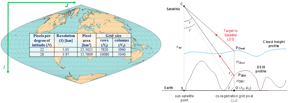
The geo-projection is done with respect to a fixed sinusoidal grid, using the Sanson-Flamsteed projection (Figure 1). This projection has been chosen mainly because of its equal area properties and the flexibility of its pixels size configuration (set by default as close as possible to the nominal nadir ground resolution of the instrument, i.e. at approx. 4km).

In order to achieve an accurate geo-projection to this grid, the 3MI L1B to L1C processor uses a strategy of 'inverse' location from the pixels centre of a defined overlap area back to the instrument detector surface (see Figure 4). The 'inverse' location procedure aims at calculating the coordinates (generally fractional) of the focal plane pixel 'C' associated to a target pixel 'O'. The use of this technique also allows to perform the so-called parallax correction at no additional cost, making the end-to-end processing of co-registered and parallax corrected signals both accurate and efficient.

Figure 1 on the right shows fixed sinusoidal grid (Sanson-Flamsteed projection) is the chosen reference for the co-registration. By default, the grid point size is close to the nominal Nadir ground resolution of the instrument (4km) and on the left shows, with the Inverse location strategy, a particular line of sight (LOS) angle γ is defined from an arbitrary target 'O' on the Earth surface back to the focal plane instrument, thus deriving the fractional coordinates focal plane pixel which would have sensed the target O, the parallax correction of the LOS angle γ to γ’ the geodetic height of target O is taken into account using ancillary information (geoid, digital elevation model terrain altitude or cloud top or scattering layer height).

Re-gridding (co-registration) and the concept of 'overlaps'

The processing has to be carried out such that chunks of data ('granules') of a configurable amount, i.e. during a configurable time of sensing, can be processed and disseminated to the end-user with high timeliness, as required by the EPS-SG overall end-user requirements.

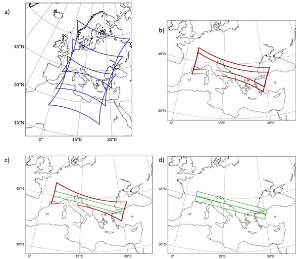
Taking as a reference the size of the 3MI-VNIR footprint, the maximum amount of views of the same target that the instrument is capable of acquiring is set to 14. This is the minimum input view buffer which defines an area on the target co-registration grid (Figure 4), which we call one 'overlap', and for which all the grid pixels have been seen by all spectral acquisitions, and under all observation angles ('views'). The co-registration of the measurements to the overlap generates the shortest possible level 1C data granule. The actual overlap area is a subset of the maximum available overlap area. and it is derived by a portion of the VNIR IFOV, so that the next overlap area is adjacent to the next one.

For a specific spectral band and a specific viewing direction, the signal co-registered to 'O' is then computed using bi-linear (default) or bicubic interpolation of the surrounding detector pixel read-out signals l,p (provided by the level 1B product) to the fractional detector coordinates l_f,p_f.

Figure 2 is the a) Example of a first, middle and last IFOV (view 1, 7 and 14) with a common overlap area. b) Two consecutive maximum-intersection areas for the first 14 IFOV of a) and when removing the first view and adding the next view (view 2 to 15). c) A single maximum-overlap like in b) (red) and the common overlap area for view 1 to 14 named one “overlap” (green). It is defined such that the overlap related to view 2 to 15 is perfectly adjacent (d) and multiple processing of the same reference grid-point on ground is avoided.

Provision of angular information

Encoding the full satellite and solar angular information for all pixel of the overlaps would, therefore, significantly increase the size of the level-1C product. Therefore a dedicated fitting algorithm based on a simplified orbital model has been developed for the satellite angles. The user of the level-1C product is then provided with a small set of coefficients and a set of dedicated functions to reconstruct the elevation and azimuth satellite angles.

Co-location of ancillary data

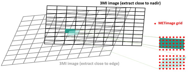
The L1C processor contains a module for the co-location of ancillary information. For the 3MI level-1C product the most important co-location is with METimage observations, provided at a significantly higher spatial sampling (500m) than the one of 3MI. In this case the co-location method of choice is a 'point-in-polygon' collection of METimage data, where each METimage measurement is treated as a dimensionless point measurement and a set of METimage measurements are identified with one 3MI observation (Figure 3). Binary cloud-flag information from VII (cloudy/non-cloudy pixel information) can then be aggregated to a geometrical cloud-fraction (CFR) associated with one 3MI pixel, and additional ancillary information (like cloud top-height (CTH) or radiances) can be provided as geometric mean or variance values.

METimage’s sub-pixel information is provided in the EPS-SG ground segment to the L1C processing chain by an intermediate 'fast-track' L2 product dedicated for the 3MI L1 and L2 processing chain. This intermediate product provides a cloudy or non-cloudy pixel flag, a CTH estimate and radiances information from the METimage channels at 555, 865 and 2130nm.

Figure 3 shows 3MI footprints for co-location with ancillary data are represented as polygons with four vertices around the centre pixel location (provided by the level-1b processing). The grey and black polygons show a small subset of pixels of the IFOV close to the nadir point (black) and towards one edge of the IFOV (grey). Here we present the case or a point in polygon co-location approach (see in-lay at the bottom), which is predominantly used in the L1C processor for co-location of METimage observations taken at significantly higher sampling (500m) and treated as points. Depending on the 3MI observation geometry, the projection of the detector pixel polygon on ground can cover quite different areas (lower right side), which then affect the selection of associated METimage point observations and, therefore, the aggregated METimage ancillary data result.

Estimate of the radiometric error

The overall radiometric error of the co-registered and resampled radiances provided in the L1C product consist of four components:

1. The instrument noise.
2. The uncertainty in the instrument absolute radiometric knowledge.
3. The uncertainty knowledge of the observation geometry per acquisition. This uncertainty has three components:
   • the pointing error of the instrument;
   • the position error of the satellite, and;
   • the error of the inverse geometrical model.
4. The error introduced by spatial aliasing and the associated interpolation method when resampling the data towards the target.

All of these error components impact directly or indirectly the radiometry, especially when the target is not spatially homogeneous.

The L1C product will provide an estimate of those contributors to the radiometric error which can be used as randomly distributed errors (point 1). An estimate of the error introduced by spatial aliasing (essentially the insufficient sampling of the PSF) and resampling (interpolation), point 4) is derived from the sub-pixel in-homogeneity information provided by METimage. The spatial aliasing error is derived such that it can be used as an additional noise component added to the instrument detector noise and used for data-assimilation. This estimate is carried out also comparing the co-registered radiances with a 'perfect' L1C dataset, for which the TOA radiances are calculated using directly the co-registration fixed-grid and are not interpolated from the instrument native ground pixel grid (i.e. no re-gridding error is involved for the 'perfect/ L1C product).

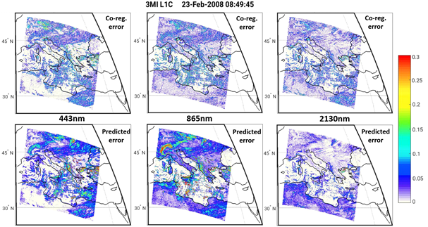
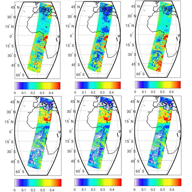
Results and test dataset availability

Figure 5 shows reflectance factor values for top-of-atmosphere radiance values I for the same orbit and, therefore, for the same co-located observation geometries for the 443nm of the VNIR detector (top row) and for the observation geometries of the SWIR detector (bottom row).