16 February 2023
03 August 2020
The purpose of the study was to develop and demonstrate tools to statistically model and monitor the degradation and evolution of operational LEO optical sensors, such as OLCI and SLSTR, using the earth as a reference source, without reference to on-board devices.
Five areas of study were included, two focused on using Level 0 count data for tracking absolute calibration drift and for monitoring the degradation of the on-board diffusers. The other three used Level 1 radiance data for monitoring Signal to Noise Ratio, Relative Gain and non-linear behaviour in individual detector responses.
Among the benefits observed were the fact that this approach provided very high temporal sampling of parameters of interest so that issues could be identified as they occur and that features were identified that could not be determined by the on-board systems.
Objectives
Using operational observations only, develop, implement, document and validate algorithms to:
- At Level-0
- Model radiometric calibration drift.
- Assess the ageing of on-board calibration devices.
- At Level-1
- Assess Signal to-Noise-Ratio (SNR).
- Derive individual detector Relative Gains.
- Assess instrument Non-Linearity.
Overview
Introduction
The absolute calibration and the radiometric evolution of an optical system are usually delegated to on-board devices, such as solar diffusers, that are periodically exposed to solar radiation in order to monitor the radiometric response of the instrument. Observations of the solar diffuser are also used for the estimation of SNR and relative gain. In case of missing on-board calibration devices, a space system can be monitored and calibrated with some well-known vicarious techniques (e.g. Rayleigh scattering, observation of Pseudo-Invariant Desert Sites, Deep Convective Clouds, etc).
However, an alternative method, particularly suited to global datasets, is based on the idea of using the whole earth as a reference dataset. The key assumption is that the mean properties of the earth are nearly constant over the sensor lifetime (~10 years) — the underlying assumption being the need for stability for the spectral bands that have to be monitored over extended time periods. The goal of this activity was to explore alternative techniques for assessing the evolution of operational optical payloads, such as OLCI and SLSTR, on this basis.
Results
The software was developed, installed at EUMETSAT and run on 'live' OLCI and SLSTR data. While a 12-month demonstration phase was originally planned, a longer than expected development phase meant that this was shortened to six months. The software will continue to run at EUMETSAT until a full year of data collection is completed.
Overall, the study has proved the potential for assessing the evolution of operational optical payloads without using any on-board device, and relying only on operational observations. It has considerable power to inform on, and improve, the quality of data from existing sensors, and represents an interesting possibility for integration into the routine monitoring of future sensors.
A brief summary of results is outlined below. For full details of each of these techniques and their results see Study Documents
Level 0 – OLCI
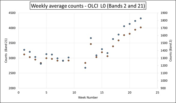
The Level 0 data, generated and aggregated at the weekly level, showed coherent patterns of behaviour over a five-month period (Figure 1), which suggests a reference curve for both the calibrator drift and the absolute calibration drift could be defined with this technique. Data collection needs to continue to a minimum of at least one year to fully assess the methodology. However, the approach looks very promising as an alternative/complement to traditional calibration.
Level 0 – SLSTR
This code was prototyped and showed promising results, but could not be fully validated within the timeframe of the study.
Level 1 – OLCI
All three Level 1 algorithms gave very useful results, which were part-validated by the on-board devices, but also raised some important questions on the results currently obtained by these devices and potential issues with either the methodologies being used or the sensor operation.
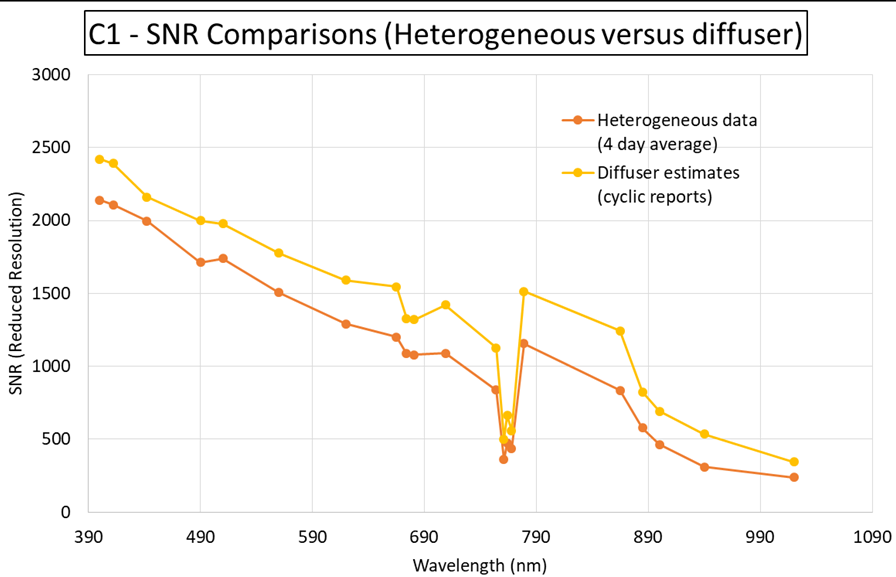
SNR: Weekly SNR estimates were consistent through time and across all bands (Figure 2) but this technique gave a lower SNR than the diffuser data, although relative differences were similar (Figure 3). Differences between cameras were consistent with Cyclic Reports. As absolute validation against the diffuser was not possible, a single pre-launch curve and results for homogeneous snow scenes were used, which gave results in line with the heterogeneous images.

Relative Gain: The relative gain differences observed consisted of two types. The first type were simple deviations from normal for single detectors that could be seen by both the heterogeneous imagery and the on-board diffuser, and could be easily removed.
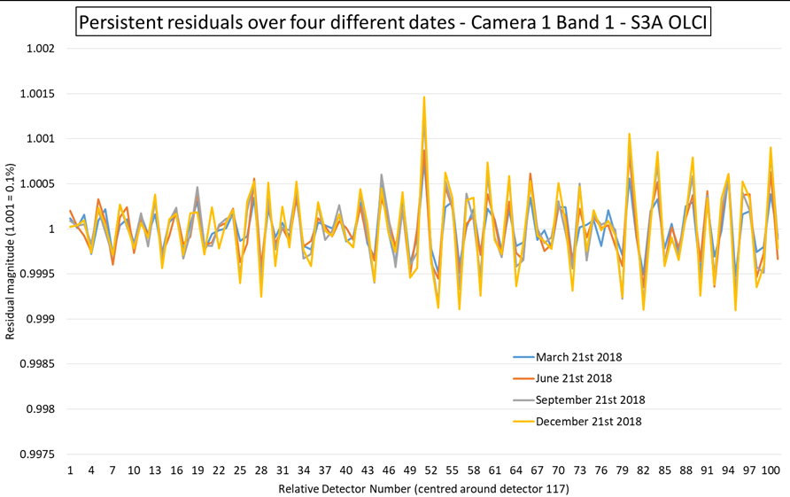
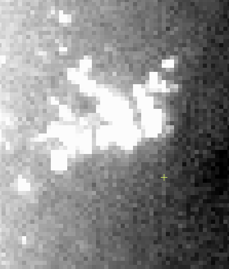
The second type, persistent residuals — present for at least two years, not detected by the on-board diffuser and which could not be corrected — were also observed (Figure 4). Validation using simple image analysis showed that the observed features are also visible in the imagery (Figures 5 and 6).

Non-Linearity: The relative gain provides a magnitude for the residual striping using the entire radiance range. The non-linearity looks at the same relative gain residual striping data but in small radiance bins rather than using the whole radiance range. Radiance specific changes in the residuals could be identified and, hence, possible causes of the residuals (multiplicative, mixed, or additive) identified.
Level 1 – SLSTR
The SLSTR SNR algorithm produced good results. The generated data clouds provided a lot of detail which suggested that this sensor does not have a simple response and that its noise profile is by no means a standard shot noise limited curve. No other methodology can derive this information with this level of detail.